Introduction
One of the most exciting applications in the realm of industrial automation is motion control. It never gets old seeing your machines flying and doing everything nice and smooth.
When it comes to SIEMENS motion control, one of the solutions is the technology object. It is mostly useful when it comes to multi-axis applications with relatively lower dynamic performance requirements. Of course, this relatively lower dynamic performance is compared to the high dynamic performance of EPOS which I will introduce in another article. Mastering the technology object is the pathway to an advanced automation engineer.
So let’s get started.
What is Technology Object
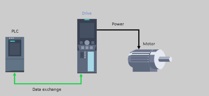
Technology object is a SIEMENS solution to address automation applications with abstracted software models and standard interfaces with a wide range of hardware.
Below is the configuration view of a technology object.
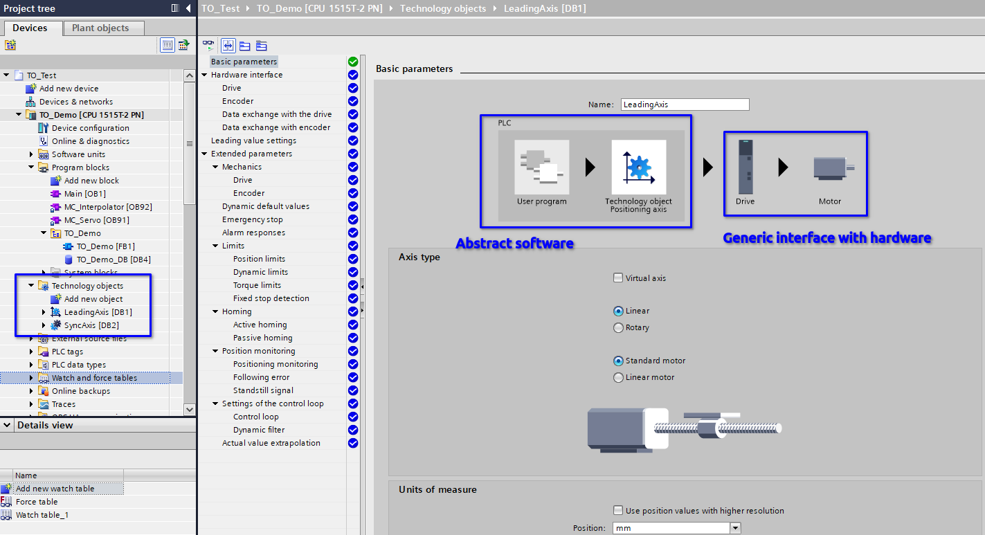
As shown in the configuration view, anything related to the logic of the motion control and the performance requirements are done in the PLC. Afterwards, any kind of motion control products SIEMENS or not can be connected to the technology object and execute the motion control tasks as long as the motion control product is able to deliver the torque, the speed, etc.
Benefits of the Technology Object
Among all the benefits of the technology object, I will say the biggest is the flexibility. As motion control tasks become complex, having all your motion control logic in one place with all the clear programs and comments becomes crucial and with a technology object you can easily do it.
Additionally, the technology object is a TIA portal program which means it can be managed as a software library and efficiently deployed whenever a new project comes.
Last but not the least, technology object is hardware independent so with different motion control products, you don’t need to re-program: just change the hardware interface.
Disadvantages of the Technology Object
The technology object uses quite some PLC calculation power and dedicated motion control interrupts. As motion control tasks get complex, the requirements to the PLC get higher. Though the T-CPUs can handle the challenge well, extra cost is inevitable.
Also, technology object relies on PLC communication with the motion control products. The dynamic performance is capped by the PLC scan time and the communication time. If the application requires extremely high accuracy / response, technology object won’t be able to handle it.
However, it is safe to say that most of the motion control applications are covered by the technology object as well as some other applications like PID controls, high speed counters, RFID identifications, etc.
Application Demonstration
In this application demonstration, I am focusing on three most frequent used technology objects: position axis, synchronization axis, and cam output.
The position axis will continuously run in one direction and in modulo mode (its position will reset to the start position after hitting the max).
The sync axis will gear with the position axis based on the position axis’s real time position and disengage from it after running together for some distance.
The position axis will also trigger a cam output based on the position axis’s real time position.
Adding Technology Objects to the Project
Adding a TO is easy. Simply insert it in the technology object folder of your PLC.
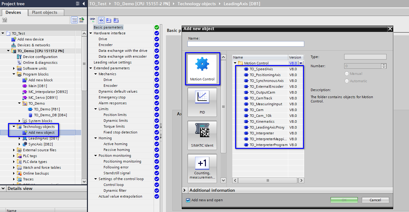
There are many different types of technology objects. In this demonstration, we will only use one position axis, one synchronous axis and one output cam.
Setting Technology Object as Simulation
In this demonstration, I am using PLCSim Advanced to run the TOs (another reason to use TO because it allows software tests without hardware support).
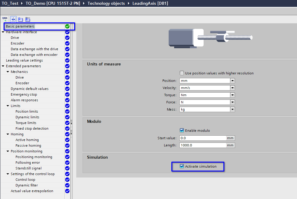
After ticking the box in the above picture, the TO will be simulated by PLCSim Advanced and no hardware support like drives and motors are necessary anymore.
Assign Leading Axis to Sync Axis
Since we are doing axis synchronization, we need to tell the sync axis who to follow. This is done below.
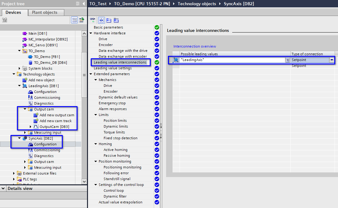
One more thing to notice is the output cam is not a stand alone TO in the TO folder. It resides in the output cam folder of another axis.
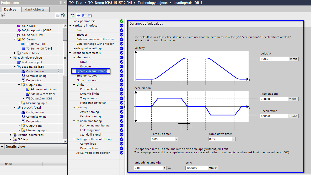
Configuring Dynamic Parameters
Though there is no hardware, it is useful to verify that logically / ideally the motion profile can fulfill the application requirements. Hence in simulation mode, the TOs will run with the same motion profile that later the drive products will follow. Below shows how to configure the motion profile.
Programming the Motion Control Application
The programming is this demonstration is quite simple. However, there are many advanced programming skills and approaches that come with the TO applications. I can’t possibly exhaust them in such a short article. Instead, I’ll just provide the simple program that I made to produce this demonstration.
FUNCTION_BLOCK "TO_Demo"
{ S7_Optimized_Access := 'TRUE' }
VERSION : 0.1
   VAR_INPUT
      i_Enable : Bool;
      i_Home : Bool;
      i_Reset : Bool;
   END_VAR

   VAR_OUTPUT
      io_LeadingAxis {InstructionName := 'TO_PositioningAxis'; LibVersion := '8.0'} : TO_PositioningAxis;
      io_SyncAxis {InstructionName := 'TO_SynchronousAxis'; LibVersion := '8.0'} : TO_SynchronousAxis;
      io_CamOutput {InstructionName := 'TO_OutputCam'; LibVersion := '8.0'} : TO_OutputCam;
   END_VAR

   VAR
      s_LeadingAxisPower {InstructionName := 'MC_POWER'; LibVersion := '8.0'; S7_SetPoint := 'False'} : MC_POWER;
      s_LeadingAxisHome {InstructionName := 'MC_HOME'; LibVersion := '8.0'} : MC_HOME;
      s_LeadingAxisReset {InstructionName := 'MC_RESET'; LibVersion := '8.0'} : MC_RESET;
      s_LeadingAxisMoveV {InstructionName := 'MC_MOVEVELOCITY'; LibVersion := '8.0'; S7_SetPoint := 'False'} : MC_MOVEVELOCITY;
      s_SyncAxisPower {InstructionName := 'MC_POWER'; LibVersion := '8.0'} : MC_POWER;
      s_SyncAxisGearIn {InstructionName := 'MC_GEARIN'; LibVersion := '8.0'} : MC_GEARIN;
      s_SyncAxisGearOut {InstructionName := 'MC_GEAROUT'; LibVersion := '8.0'} : MC_GEAROUT;
      s_SyncAxisHome {InstructionName := 'MC_HOME'; LibVersion := '8.0'} : MC_HOME;
      s_CamOutput {InstructionName := 'MC_OUTPUTCAM'; LibVersion := '8.0'} : MC_OUTPUTCAM;
   END_VAR


BEGIN
	REGION Leading Axis

	    #s_LeadingAxisPower(Axis      := #io_LeadingAxis,
	                        Enable    := #i_Enable,
	                        StartMode := 1,
	                        StopMode  := 0);

	    #s_LeadingAxisHome(Axis     := #io_LeadingAxis,
	                       Execute  := #i_Home,
	                       Position := 0,
	                       Mode     := 0,
	                       Sensor   := 0);

	    #s_LeadingAxisReset(Axis    := #io_LeadingAxis,
	                        Execute := #i_Reset,
	                        Restart := FALSE);

	    #s_LeadingAxisMoveV(Axis    := #io_LeadingAxis,
	                        Execute := #s_LeadingAxisPower.Status);

	END_REGION

	REGION Sync Axis

	    #s_SyncAxisPower(Axis      := #io_SyncAxis,
	                     Enable    := #i_Enable);

	    #s_SyncAxisGearIn(Master           := #io_LeadingAxis,
	                      Slave            := #io_SyncAxis,
	                      Execute          := #io_LeadingAxis.ActualPosition >= 100);

	    #s_SyncAxisGearOut(Slave                := #io_SyncAxis,
	                       Execute              := #io_LeadingAxis.ActualPosition >= 400,
	                       SlavePosition        := 310,
	                       SyncProfileReference := 0);

	    #s_SyncAxisHome(Axis     := #io_SyncAxis,
	                    Execute  := #io_LeadingAxis.ActualPosition > 800 OR #i_Home,
	                    Position := 0,
	                    Mode     := 0,
	                    Sensor   := 0);

	END_REGION

	REGION Cam Output

	    #s_CamOutput(OutputCam   := #io_CamOutput,
	                 Enable      := #s_LeadingAxisMoveV.InVelocity,
	                 OnPosition  := 500,
	                 OffPosition := 600);

	END_REGION
END_FUNCTION_BLOCK
Conclusion
This article introduces the concept of the technology object and provides a simple demonstration of it with one position axis, one synchronization axis and one output cam. The TO applications are so complex and flexible that this article can only provide a glimpse into this exciting world.
TO provides a software solution to complex motion control tasks and is the most important pathway for an automation engineer to reach the advanced level. I welcome any question about the technology object.