Introduction
Trace is the most important commissioning tool in TIA Portal and it offers many cool features that can simplify our analytical works. However, I can barely see people using any more trace features than the most basic continuous trace even though they should.
In this article, I am going to introduce and demonstrate some features that everyone should know and at times they can be very handy helping us figure out issues.
How To Use Continuous Trace
Trace is extremely easy to get started. Under each PLC that supports the trace feature, there is a trace folder. Simply add a trace to start with and you can specify the signals that you want to trace, how you want the sampling to be done and how many sampling points, etc.
This is the most basic way to use trace.
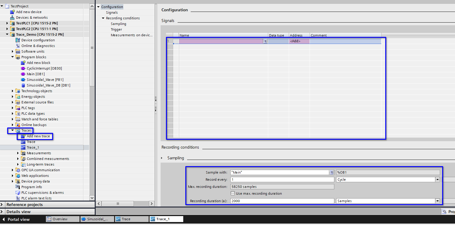
Trace With A Different Sampling Time
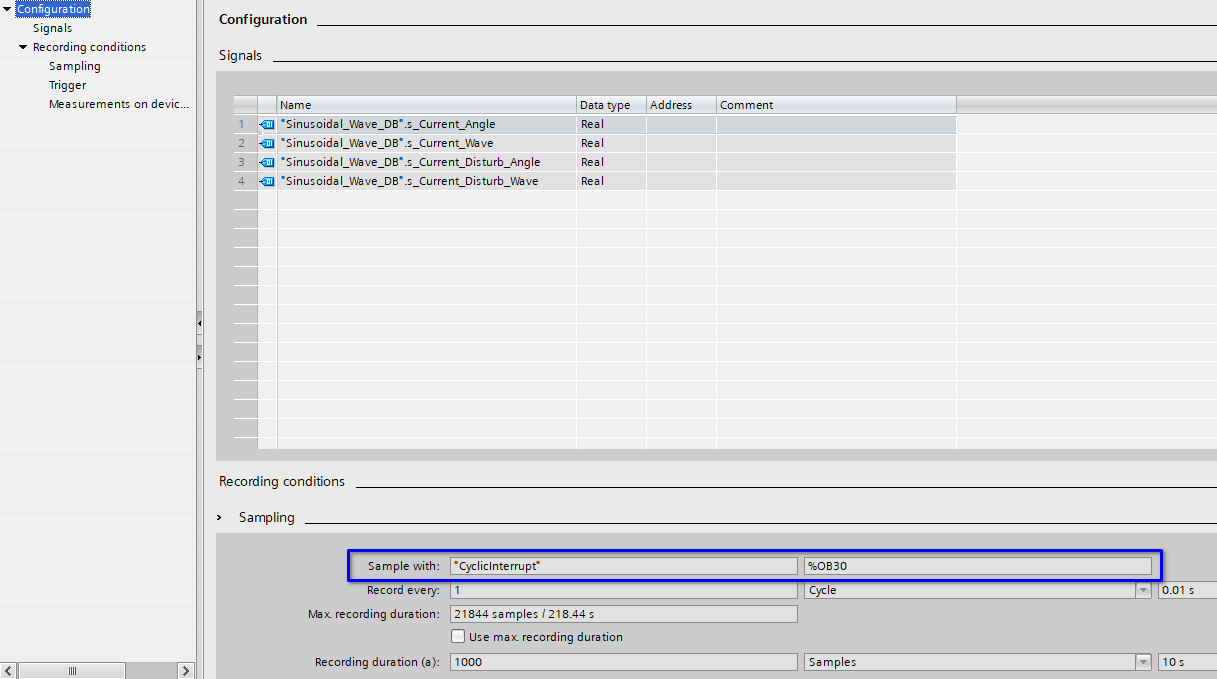
In some special cases you may want to have a higher sampling rate or your samples are done with fixed time intervals so you can do further analysis easier. This can be achieved with specifying a different sampling organization block.
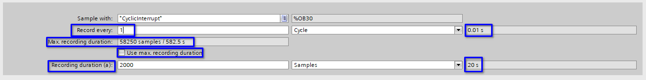
In the trace configuration page select “Sampling” and you can specify the OB that you want to sample with (of course you need to create the OB in the program folder first).
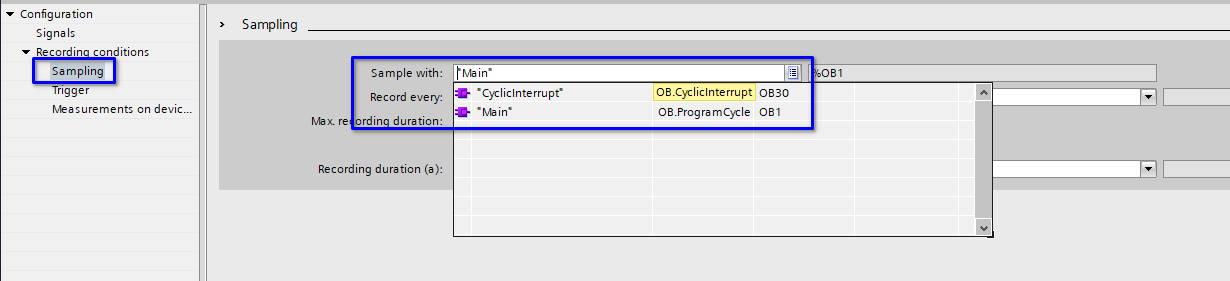
If the sampling OB executes with a fixed interval (i.e. periodic interrupt OB), then you can accurately specify how many sampling points you want and the sampling duration.
This will enable advanced analyzing features that I will introduce later in this article.
One thing to note here is that higher trace sampling rate only means you can see the signal states with a higher resolution. It doesn’t affect how your program responds to the signal unless you execute your programs at the same rate.
Trigger Trace
Trigger trace is arguably the most useful trace feature.
It is available if you configure your trace to be triggered on a tag, specify the tag and the tag condition(s).
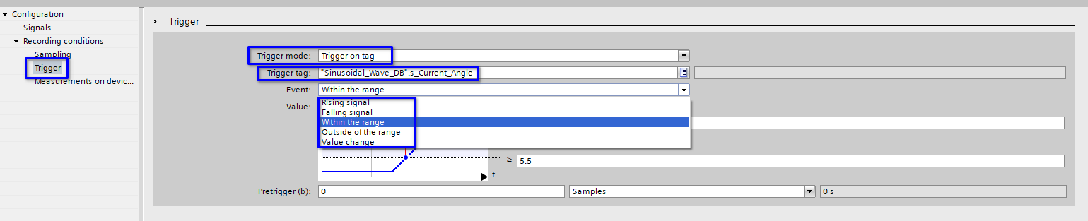
In many cases, we want to “catch the moment”. Instead of continuously run the trace and hope to catch the issue, we can simply set up the appropriate trigger trace conditions and the traced signals and let it run. Trigger trace will catch the moment for us and keep it in the PLC until we come back and get it.
You can even configure pre-trigger samplings to learn what happened before the trigger happened to get a better understanding of the issue.
In the below demonstration, I configured the trace to only start when the tag “Sinusoidal_Wave_DB”.s_Current_Angle is bigger than 5.5, the sampling rate is 0.01s and the sampling will last for 10s.
With trigger trace, I don’t need to manually catch the specific time, instead trace will do all the job for me much more accurately.
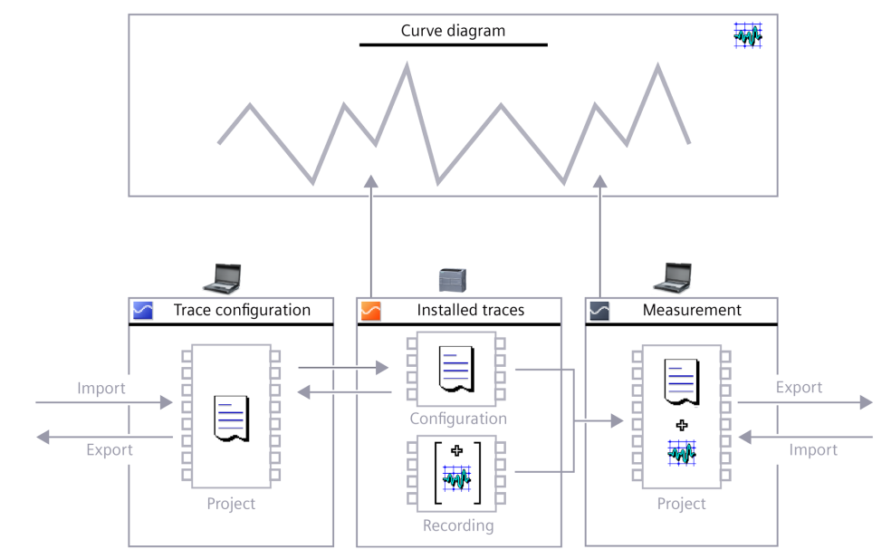
Post Trace Data Analysis
In many cases we not only want to have traces of signals but also want to find certain characters of them or the correlations between them. Many people will write programs to let the PLC calculate this information and trace the result. However, there is a better way to do it.
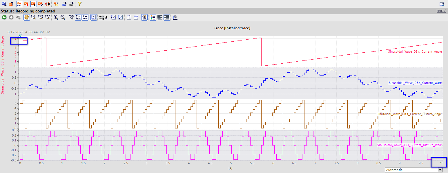
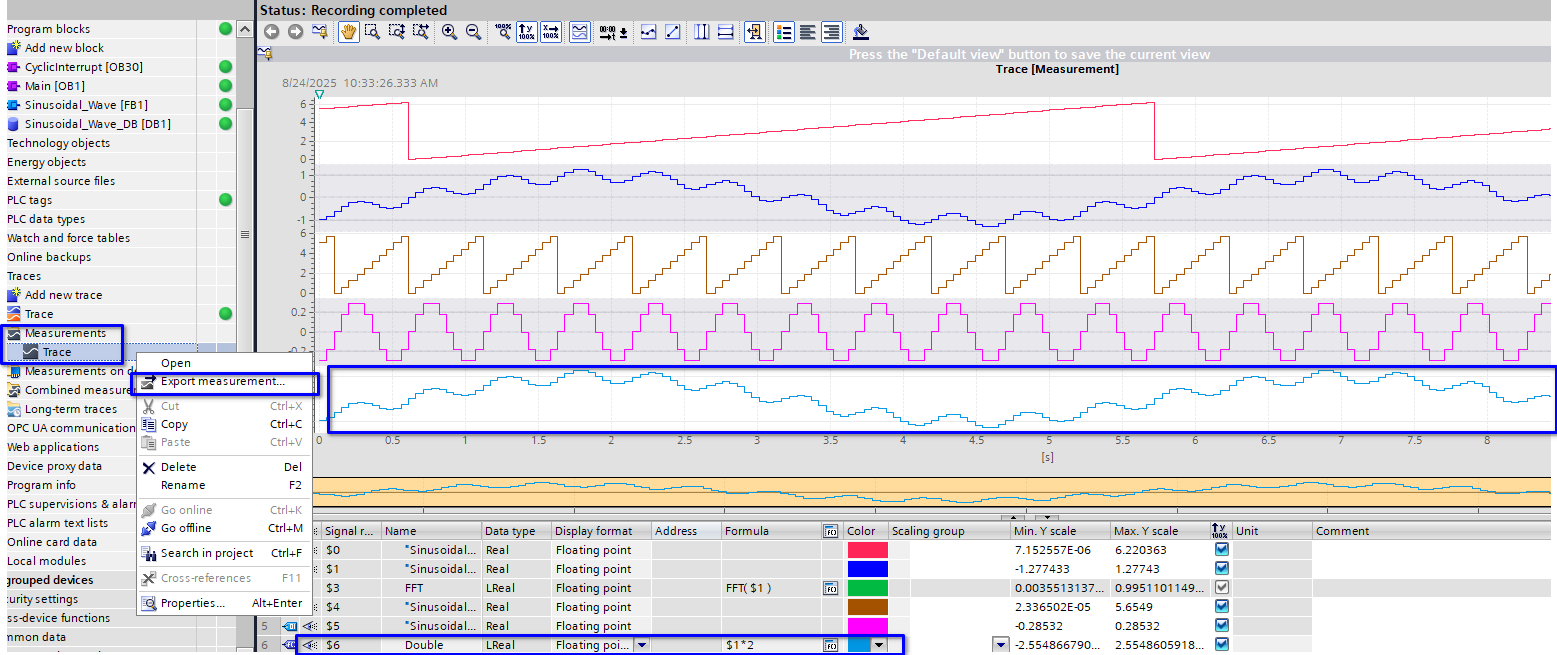
In the last example, I have traced a 0.2 Hz 1.0 amplitude sinusoidal signal compounded by a 2 Hz 0.3 amplitude disturbance. If I want to know the frequency components of this signal, I’ll need to perform a FFT (Fast Fourier Transformation) on the traced signal which is too much for the PLC to calculate in real time.
The good news is I don’t have to. The trace function of TIA Portal has the ability to perform FFT and Bode analysis. As shown in the below picture, by simply applying FFT on the $1 signal which is the compounded sinusoidal signal, I can easily see that the base frequency is 0.2 Hz and the highest fraction of the harmonics is 2 Hz.
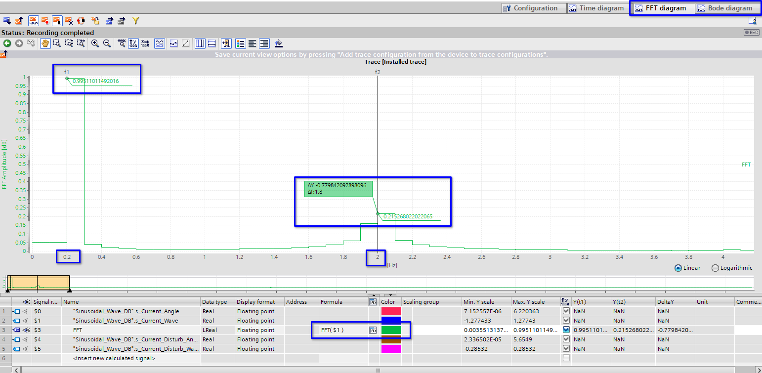
And this is easily done by inserting another calculated signal in the trace and apply the calculation formula.
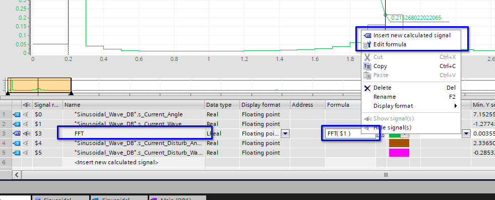
However you want to analyze your traced signals, simply put the formula here and TIA Portal can calculate for you.
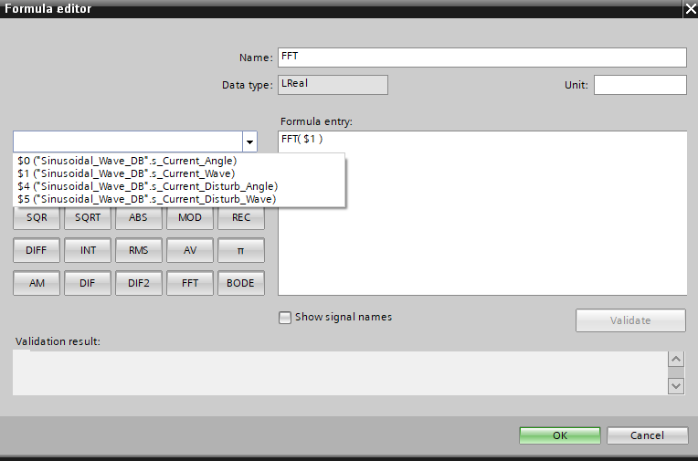
There is one thing to note that since analysis like FFT requires fixed sampling intervals, you need to run your trace with a cyclic interrupt OB instead of the default OB1, otherwise FFT can’t work.
Even More
The above trace functions are most likely to be used in our daily jobs. The below functions are game changers that can swoop in and save the day.
Long Trace
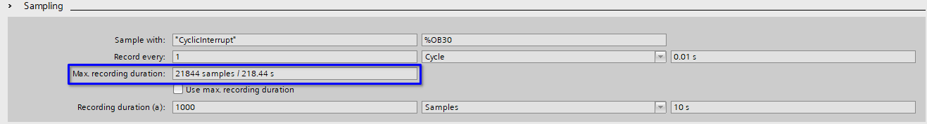
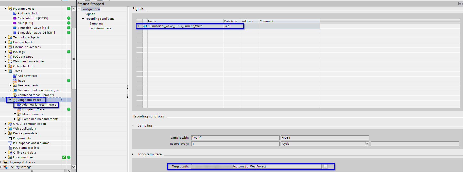
The duration of a standard trace is limited to the PLC’s memory. For example, my demo project PLC’s maximum duration is 218.44s with the cyclic interrupt sampling rate.
What if we want to trace a signal for hours? The answer is the long trace. Introduced since TIA Portal V19, the long trace feature allows you to run trace for the max amount of time possible and the limitation is your PC’s storage capacity.
Say goodbye to proprietary software like PLC Observer.
Move A Trace
Often we want to send our trace to others and most frequently people will make a screenshot of the trace. However, the screenshot loses lots of information and the recipient can’t check the details.
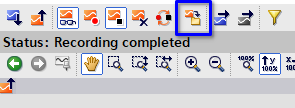
The proper way to move a trace is to create measurement or export the trace. Since I prefer providing as comprehensive information as possible, I normally use measurements. After getting the ideal trace results, simply click the below button and TIA Portal will create the measurement out of your trace.
After doing so, there are a few things that you can do.
- Export the trace. The trace will be exported as a .ttrecx file that contains all the details.
- Add new calculations to your trace whenever you want.
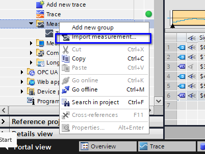
You can even add other calculations after importing a trace file to the measurements hence it is easy to analyze other people’s trace in your TIA Portal.
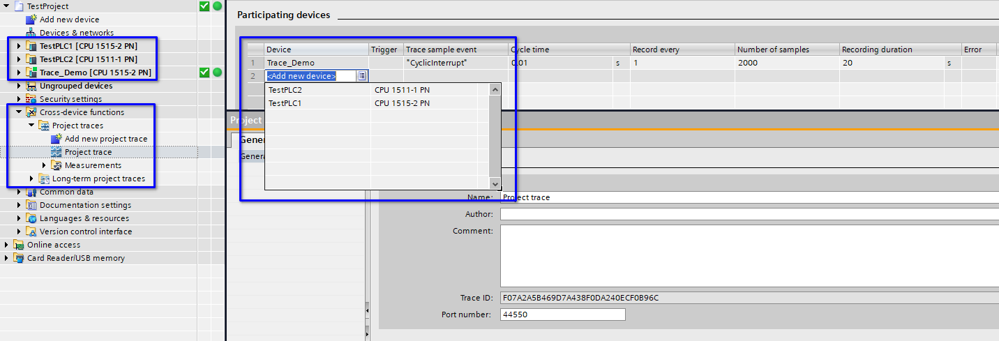
Cross Project Trace
This is another amazing feature. You can set up a project-wise trace that can trace multiple PLCs’ signals at the same time following the below picture. This feature is particularly helpful if you have multiple PLCs in a project and there are issues regarding their coordinations.
Conclusion
Though everyone knows about the trace function of TIA Portal, most of the control engineers only use the very basic functions. This article introduces the advanced features of trace and their applicable scenarios.
In Addition
The program that I used to generate sinusoidal signals with disturbance is below.
FUNCTION_BLOCK "Sinusoidal_Wave"
{ S7_Optimized_Access := 'TRUE' }
VERSION : 0.1
   VAR_INPUT
      i_Enable : Bool;
      i_Reset : Bool;
      i_Period : Time;   // Period in ms, 1000ms minimum
      i_Amplitude : Real;
      i_Resolution : Time;   // 50ms minimum
   END_VAR

   VAR
      s_UpdateTimer {InstructionName := 'TON_TIME'; LibVersion := '1.0'; S7_SetPoint := 'False'} : TON_TIME;
      s_Disturb_UpdateTimer {InstructionName := 'TON_TIME'; LibVersion := '1.0'} : TON_TIME;
      s_Current_Angle { S7_SetPoint := 'True'} : Real;
      s_Current_Wave : Real;
      s_Current_Disturb_Angle : Real;
      s_Current_Disturb_Wave : Real;
      s_WaveConstruct : Struct
         period : Time;
         resolution_Time : Time;
         resolution_Degree : Real;
      END_STRUCT;
      s_Disturbs : Struct
         period : Time := T#500ms;
         amptitude : Real := 0.3;   // Percentage
         resolution_Time : Time := T#50ms;
         resolution_Degree : Real;
      END_STRUCT;
   END_VAR

   VAR CONSTANT
      c_2Pi : Real := 6.283186;
   END_VAR


BEGIN
	REGION Input Check

	    IF #i_Resolution < T#50ms THEN
	        #s_WaveConstruct.resolution_Time := T#50ms;
	    ELSE
	        #s_WaveConstruct.resolution_Time := #i_Resolution;
	    END_IF;

	    IF #i_Period < T#1s THEN
	        #s_WaveConstruct.period := T#1s;
	    ELSE
	        #s_WaveConstruct.period := #i_Period;
	    END_IF;

	END_REGION

	REGION Reset Wave Generation

	    IF #i_Reset THEN
	        #s_Current_Angle := 0;
	        #s_Current_Wave := 0;
	    END_IF;

	END_REGION

	REGION Update Intervals and Values

	    #s_UpdateTimer(IN := #i_Enable AND NOT #i_Reset,
	                   PT := #s_WaveConstruct.resolution_Time);

	    #s_Disturb_UpdateTimer(IN := #i_Enable AND NOT #i_Reset,
	                           PT := #s_Disturbs.resolution_Time);

	    #s_WaveConstruct.resolution_Degree := #c_2Pi / DINT_TO_REAL((TIME_TO_DINT(#s_WaveConstruct.period) / TIME_TO_DINT(#s_WaveConstruct.resolution_Time)));

	    #s_Disturbs.resolution_Degree := #c_2Pi / DINT_TO_REAL(TIME_TO_DINT(#s_Disturbs.period) / TIME_TO_DINT(#s_Disturbs.resolution_Time));

	END_REGION

	REGION Calculate the Wave

	    IF #s_Disturb_UpdateTimer.Q THEN
	        #s_Current_Disturb_Angle += #s_Disturbs.resolution_Degree;

	        IF #s_Current_Disturb_Angle > #c_2Pi THEN
	            #s_Current_Disturb_Angle -= #c_2Pi;
	        END_IF;

	        RESET_TIMER(#s_Disturb_UpdateTimer);

	    END_IF;

	    IF #s_UpdateTimer.Q THEN
	        #s_Current_Angle += #s_WaveConstruct.resolution_Degree;

	        IF #s_Current_Angle > #c_2Pi THEN
	            #s_Current_Angle -= #c_2Pi;
	        END_IF;

	        RESET_TIMER(#s_UpdateTimer);

	    END_IF;

	    #s_Current_Disturb_Wave := SIN(#s_Current_Disturb_Angle) * #i_Amplitude * #s_Disturbs.amptitude;

	    #s_Current_Wave := SIN(#s_Current_Angle) * #i_Amplitude + #s_Current_Disturb_Wave;

	END_REGION
END_FUNCTION_BLOCK